Earth's Magnetic Field Affects Apex

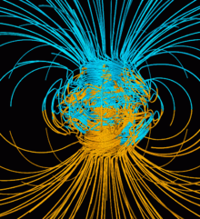
Magnetic field that extends from the Globe's outer and inner core to where it meets the solar air current

Estimator simulation of Earth'due south field in a period of normal polarity between reversals.^[1] The lines represent magnetic field lines, blueish when the field points towards the center and yellow when away. The rotation axis of Earth is centered and vertical. The dense clusters of lines are within Earth'southward core.^[2]

Earth's magnetic field, as well known every bit the geomagnetic field, is the magnetic field that extends from Earth'southward interior out into space, where it interacts with the solar wind, a stream of charged particles emanating from the Sun. The magnetic field is generated by electric currents due to the movement of convection currents of a mixture of molten iron and nickel in Globe'due south outer cadre: these convection currents are acquired by heat escaping from the core, a natural procedure chosen a geodynamo. The magnitude of Earth'south magnetic field at its surface ranges from 25 to 65 μT (0.25 to 0.65 G).^[3] Every bit an approximation, it is represented by a field of a magnetic dipole currently tilted at an angle of about 11° with respect to Earth'southward rotational axis, as if there were an enormous bar magnet placed at that angle through the center of Globe. The North geomagnetic pole actually represents the Due south pole of Globe's magnetic field, and conversely the South geomagnetic pole corresponds to the northward pole of Earth's magnetic field (because opposite magnetic poles concenter and the north stop of a magnet, like a compass needle, points toward Earth's South magnetic field, i.east., the N geomagnetic pole well-nigh the Geographic Northward Pole). As of 2015, the Northward geomagnetic pole was located on Ellesmere Island, Nunavut, Canada.

While the Northward and Due south magnetic poles are normally located near the geographic poles, they slowly and continuously move over geological time scales, but sufficiently slowly for ordinary compasses to remain useful for navigation. Still, at irregular intervals averaging several hundred thousand years, Earth's field reverses and the Northward and Southward Magnetic Poles respectively, abruptly switch places. These reversals of the geomagnetic poles leave a tape in rocks that are of value to paleomagnetists in calculating geomagnetic fields in the past. Such information in plough is helpful in studying the motions of continents and body of water floors in the process of plate tectonics.

The magnetosphere is the region to a higher place the ionosphere that is defined past the extent of Earth's magnetic field in space. Information technology extends several tens of thousands of kilometres into space, protecting World from the charged particles of the solar wind and cosmic rays that would otherwise strip away the upper atmosphere, including the ozone layer that protects Earth from the harmful ultraviolet radiation.

Significance [edit]

Globe'due south magnetic field deflects most of the solar current of air, whose charged particles would otherwise strip abroad the ozone layer that protects the Earth from harmful ultraviolet radiation.^[four] I stripping mechanism is for gas to exist caught in bubbles of magnetic field, which are ripped off past solar winds.^[v] Calculations of the loss of carbon dioxide from the atmosphere of Mars, resulting from scavenging of ions by the solar wind, indicate that the dissipation of the magnetic field of Mars caused a about total loss of its temper.^[6] ^[vii]

The written report of the past magnetic field of the Globe is known as paleomagnetism.^[8] The polarity of the Earth's magnetic field is recorded in igneous rocks, and reversals of the field are thus detectable as "stripes" centered on mid-bounding main ridges where the sea floor is spreading, while the stability of the geomagnetic poles between reversals has allowed paleomagnetism to runway the past movement of continents. Reversals also provide the basis for magnetostratigraphy, a manner of dating rocks and sediments.^[9] The field likewise magnetizes the crust, and magnetic anomalies can be used to search for deposits of metal ores.^[10]

Humans have used compasses for direction finding since the 11th century A.D. and for navigation since the 12th century.^[11] Although the magnetic declination does shift with time, this wandering is slow plenty that a simple compass can remain useful for navigation. Using magnetoreception, various other organisms, ranging from some types of bacteria to pigeons, use the World's magnetic field for orientation and navigation.

Characteristics [edit]

At any location, the Globe'south magnetic field tin can be represented past a three-dimensional vector. A typical procedure for measuring its direction is to utilize a compass to decide the direction of magnetic Due north. Its angle relative to true North is the declination ( $D$ ) or variation. Facing magnetic N, the angle the field makes with the horizontal is the inclination ( $I$ ) or magnetic dip. The intensity ( $F$ ) of the field is proportional to the force information technology exerts on a magnet. Another common representation is in $X$ (North), $Y$ (Eastward) and $Z$ (Down) coordinates.^[12]

Mutual coordinate systems used for representing the Earth's magnetic field.

Intensity [edit]

The intensity of the field is often measured in gauss (G), but is by and large reported in microteslas (μT), with 1 G = 100 μT. A nanotesla is besides referred to as a gamma (γ). The Globe's field ranges between approximately 25 and 65 μT (0.25 and 0.65 G).^[thirteen] By comparing, a strong refrigerator magnet has a field of near 10,000 μT (100 G).^[14]

A map of intensity contours is called an isodynamic chart. As the Earth Magnetic Model shows, the intensity tends to decrease from the poles to the equator. A minimum intensity occurs in the South Atlantic Anomaly over South America while there are maxima over northern Canada, Siberia, and the coast of Antarctica southward of Commonwealth of australia.^[xv]

The intensity of the magnetic field is field of study to change over fourth dimension. A 2021 paleomagnetic study from the University of Liverpool contributed to a growing trunk of evidence that the Earth's magnetic field cycles with intensity every 200 million years. The atomic number 82 author stated that "Our findings, when considered alongside the existing datasets, back up the existence of an approximately 200-million-year-long bike in the strength of the Globe's magnetic field related to deep Earth processes."^[sixteen]

Inclination [edit]

The inclination is given by an angle that can presume values betwixt -90° (upwardly) to ninety° (down). In the northern hemisphere, the field points downwards. Information technology is straight downwards at the North Magnetic Pole and rotates upwards every bit the breadth decreases until it is horizontal (0°) at the magnetic equator. Information technology continues to rotate upwards until it is straight up at the South Magnetic Pole. Inclination can exist measured with a dip circle.

An isoclinic nautical chart (map of inclination contours) for the Earth'southward magnetic field is shown below.

Declination [edit]

Declination is positive for an eastward deviation of the field relative to true north. Information technology can be estimated by comparison the magnetic north–south heading on a compass with the direction of a angelic pole. Maps typically include information on the declination every bit an bending or a pocket-sized diagram showing the relationship between magnetic due north and true north. Information on declination for a region can be represented by a chart with isogonic lines (contour lines with each line representing a fixed declination).

Geographical variation [edit]

Components of the Globe's magnetic field at the surface from the World Magnetic Model for 2015.^[15]

Intensity
Inclination
Declination

Dipolar approximation [edit]

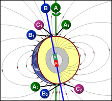
Relationship betwixt Earth's poles. A1 and A2 are the geographic poles; B1 and B2 are the geomagnetic poles; C1 (south) and C2 (northward) are the magnetic poles.

Near the surface of the Globe, its magnetic field can be closely approximated past the field of a magnetic dipole positioned at the center of the Earth and tilted at an angle of about 11° with respect to the rotational axis of the World.^[13] The dipole is roughly equivalent to a powerful bar magnet, with its south pole pointing towards the geomagnetic Northward Pole.^[17] This may seem surprising, just the north pole of a magnet is so defined considering, if allowed to rotate freely, it points roughly northward (in the geographic sense). Since the north pole of a magnet attracts the south poles of other magnets and repels the north poles, it must be attracted to the southward pole of Globe's magnet. The dipolar field accounts for 80–ninety% of the field in most locations.^[12]

Magnetic poles [edit]

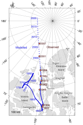
The motility of Earth's North Magnetic Pole across the Canadian arctic.

Historically, the north and south poles of a magnet were first defined by the Earth'south magnetic field, not vice versa, since one of the first uses for a magnet was as a compass needle. A magnet'southward North pole is defined as the pole that is attracted by the Earth's Northward Magnetic Pole when the magnet is suspended so it can plow freely. Since opposite poles attract, the N Magnetic Pole of the Globe is actually the south pole of its magnetic field (the place where the field is directed downwards into the Earth).^[eighteen] ^[19] ^[20] ^[21]

The positions of the magnetic poles can exist defined in at least ii ways: locally or globally.^[22] The local definition is the bespeak where the magnetic field is vertical.^[23] This can be determined by measuring the inclination. The inclination of the Earth'due south field is xc° (downwards) at the North Magnetic Pole and -xc° (upwards) at the South Magnetic Pole. The two poles wander independently of each other and are not straight opposite each other on the globe. Movements of up to 40 kilometres (25 mi) per year have been observed for the North Magnetic Pole. Over the terminal 180 years, the Northward Magnetic Pole has been migrating northwestward, from Cape Adelaide in the Boothia Peninsula in 1831 to 600 kilometres (370 mi) from Resolute Bay in 2001.^[24] The magnetic equator is the line where the inclination is zero (the magnetic field is horizontal).

The global definition of the Earth's field is based on a mathematical model. If a line is fatigued through the center of the Earth, parallel to the moment of the all-time-plumbing equipment magnetic dipole, the two positions where it intersects the Earth's surface are called the North and South geomagnetic poles. If the Earth's magnetic field were perfectly dipolar, the geomagnetic poles and magnetic dip poles would coincide and compasses would point towards them. Yet, the World'south field has a significant non-dipolar contribution, and then the poles do not coincide and compasses practise not generally point at either.

Magnetosphere [edit]

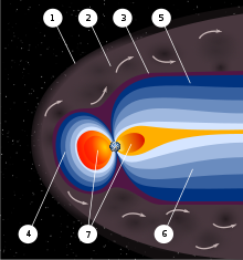
An creative person'south rendering of the structure of a magnetosphere. 1) Bow shock. 2) Magnetosheath. three) Magnetopause. 4) Magnetosphere. v) Northern tail lobe. 6) Southern tail lobe. 7) Plasmasphere.

World's magnetic field, predominantly dipolar at its surface, is distorted further out by the solar wind. This is a stream of charged particles leaving the Sun's corona and accelerating to a speed of 200 to 1000 kilometres per second. They carry with them a magnetic field, the interplanetary magnetic field (IMF).^[25]

The solar wind exerts a pressure, and if it could reach Earth's temper it would erode it. However, it is kept away past the pressure level of the Earth's magnetic field. The magnetopause, the area where the pressures rest, is the boundary of the magnetosphere. Despite its name, the magnetosphere is asymmetric, with the sunward side being near 10 Earth radii out but the other side stretching out in a magnetotail that extends across 200 Earth radii.^[26] Sunward of the magnetopause is the bow stupor, the surface area where the solar wind slows abruptly.^[25]

Inside the magnetosphere is the plasmasphere, a donut-shaped region containing low-energy charged particles, or plasma. This region begins at a height of 60 km, extends upwards to 3 or 4 Globe radii, and includes the ionosphere. This region rotates with the Earth.^[26] There are also 2 concentric tire-shaped regions, called the Van Allen radiations belts, with loftier-energy ions (energies from 0.1 to 10 MeV). The inner chugalug is i–two Earth radii out while the outer chugalug is at 4–7 Earth radii. The plasmasphere and Van Allen belts have partial overlap, with the extent of overlap varying profoundly with solar activity.^[27]

Too as deflecting the solar wind, the Earth's magnetic field deflects catholic rays, high-energy charged particles that are mostly from exterior the Solar Arrangement. Many cosmic rays are kept out of the Solar Organisation by the Sun's magnetosphere, or heliosphere.^[28] Past contrast, astronauts on the Moon risk exposure to radiation. Anyone who had been on the Moon's surface during a particularly violent solar eruption in 2005 would have received a lethal dose.^[25]

Some of the charged particles do get into the magnetosphere. These spiral around field lines, billowy dorsum and forth between the poles several times per second. In addition, positive ions slowly drift westward and negative ions drift e, giving rise to a band current. This current reduces the magnetic field at the Globe's surface.^[25] Particles that penetrate the ionosphere and collide with the atoms there give ascent to the lights of the aurorae and also emit X-rays.^[26]

The varying conditions in the magnetosphere, known as space weather, are largely driven by solar activity. If the solar wind is weak, the magnetosphere expands; while if it is strong, it compresses the magnetosphere and more of it gets in. Periods of particularly intense activity, called geomagnetic storms, tin can occur when a coronal mass ejection erupts in a higher place the Sun and sends a daze wave through the Solar Organisation. Such a moving ridge can take just two days to achieve the Earth. Geomagnetic storms can cause a lot of disruption; the "Halloween" tempest of 2003 damaged more than a third of NASA's satellites. The largest documented tempest, the Carrington Consequence, occurred in 1859. It induced currents strong enough to disrupt telegraph lines, and aurorae were reported as far south as Hawaii.^[25] ^[29]

Time dependence [edit]

Short-term variations [edit]

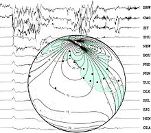
Background: a set of traces from magnetic observatories showing a magnetic storm in 2000.
Globe: map showing locations of observatories and contour lines giving horizontal magnetic intensity in μ T.

The geomagnetic field changes on time scales from milliseconds to millions of years. Shorter time scales more often than not arise from currents in the ionosphere (ionospheric dynamo region) and magnetosphere, and some changes can be traced to geomagnetic storms or daily variations in currents. Changes over time scales of a twelvemonth or more mostly reverberate changes in the World's interior, particularly the atomic number 26-rich core.^[12]

Frequently, the Earth's magnetosphere is hit past solar flares causing geomagnetic storms, provoking displays of aurorae. The short-term instability of the magnetic field is measured with the G-index.^[30]

Information from THEMIS show that the magnetic field, which interacts with the solar wind, is reduced when the magnetic orientation is aligned between Sunday and Earth – reverse to the previous hypothesis. During forthcoming solar storms, this could consequence in blackouts and disruptions in artificial satellites.^[31]

Secular variation [edit]

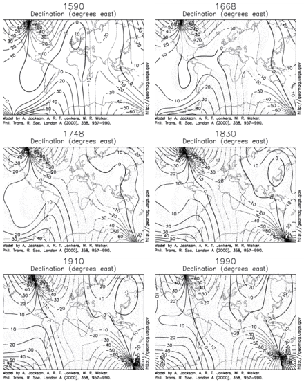
Estimated declination contours past year, 1590 to 1990 (click to run across variation).

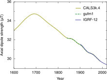
Forcefulness of the axial dipole component of World's magnetic field from 1600 to 2020.

Changes in Earth's magnetic field on a fourth dimension scale of a year or more are referred to as secular variation. Over hundreds of years, magnetic declination is observed to vary over tens of degrees.^[12] The animation shows how global declinations have changed over the last few centuries.^[32]

The direction and intensity of the dipole modify over time. Over the last 2 centuries the dipole strength has been decreasing at a rate of near six.3% per century.^[12] At this rate of decrease, the field would exist negligible in about 1600 years.^[33] However, this strength is about average for the concluding 7 thousand years, and the current rate of change is not unusual.^[34]

A prominent feature in the non-dipolar role of the secular variation is a westward drift at a rate of about 0.2° per yr.^[33] This drift is not the same everywhere and has varied over time. The globally averaged drift has been west since virtually 1400 AD simply e between nearly thou Advertising and 1400 AD.^[35]

Changes that predate magnetic observatories are recorded in archaeological and geological materials. Such changes are referred to equally paleomagnetic secular variation or paleosecular variation (PSV). The records typically include long periods of small alter with occasional large changes reflecting geomagnetic excursions and reversals.^[36]

In July 2020 scientists study that analysis of simulations and a contempo observational field model prove that maximum rates of directional modify of Globe's magnetic field reached ~ten° per twelvemonth – nigh 100 times faster than current changes and 10 times faster than previously thought.^[37] ^[38]

Studies of lava flows on Steens Mountain, Oregon, indicate that the magnetic field could take shifted at a charge per unit of up to half dozen° per day at some fourth dimension in Earth's history, which significantly challenges the pop agreement of how the World's magnetic field works.^[39] This finding was later attributed to unusual rock magnetic properties of the lava menstruation under written report, not rapid field modify, by i of the original authors of the 1995 study.^[40]

Magnetic field reversals [edit]

Geomagnetic polarity during the belatedly Cenozoic Era. Night areas announce periods where the polarity matches today'southward polarity, light areas denote periods where that polarity is reversed.

Although generally World's field is approximately dipolar, with an axis that is nearly aligned with the rotational axis, occasionally the North and South geomagnetic poles merchandise places. Bear witness for these geomagnetic reversals tin can exist institute in basalts, sediment cores taken from the ocean floors, and seafloor magnetic anomalies.^[41] Reversals occur nearly randomly in time, with intervals between reversals ranging from less than 0.1 million years to as much as 50 1000000 years. The most recent geomagnetic reversal, chosen the Brunhes–Matuyama reversal, occurred about 780,000 years ago.^[24] ^[42] A related phenomenon, a geomagnetic excursion, takes the dipole axis across the equator and and then back to the original polarity.^[43] ^[44] The Laschamp issue is an example of an excursion, occurring during the final ice age (41,000 years agone).

The by magnetic field is recorded mostly by strongly magnetic minerals, particularly fe oxides such equally magnetite, that can carry a permanent magnetic moment. This remanent magnetization, or remanence, can be acquired in more than one way. In lava flows, the direction of the field is "frozen" in minor minerals as they absurd, giving rising to a thermoremanent magnetization. In sediments, the orientation of magnetic particles acquires a slight bias towards the magnetic field as they are deposited on an ocean floor or lake bottom. This is chosen detrital remanent magnetization.^[eight]

Thermoremanent magnetization is the main source of the magnetic anomalies around mid-ocean ridges. As the seafloor spreads, magma wells upward from the pall, cools to form new basaltic chaff on both sides of the ridge, and is carried away from it by seafloor spreading. Equally it cools, it records the direction of the Earth's field. When the Earth's field reverses, new basalt records the reversed direction. The result is a series of stripes that are symmetric almost the ridge. A send towing a magnetometer on the surface of the ocean can notice these stripes and infer the historic period of the bounding main floor below. This provides information on the charge per unit at which seafloor has spread in the past.^[viii]

Radiometric dating of lava flows has been used to establish a geomagnetic polarity time scale, part of which is shown in the paradigm. This forms the basis of magnetostratigraphy, a geophysical correlation technique that can be used to date both sedimentary and volcanic sequences also as the seafloor magnetic anomalies.^[8]

Earliest appearance [edit]

Paleomagnetic studies of Paleoarchean lava in Australia and conglomerate in S Africa have concluded that the magnetic field has been present since at least about 3,450 million years ago.^[45] ^[46] ^[47]

Future [edit]

Variations in virtual centric dipole moment since the final reversal.

Starting in the belatedly 1800s and throughout the 1900s and later, the overall geomagnetic field has become weaker; the present potent deterioration corresponds to a ten–15% reject and has accelerated since 2000; geomagnetic intensity has declined almost continuously from a maximum 35% to a higher place the modern value, from circa yr 1. The charge per unit of decrease and the current forcefulness are inside the normal range of variation, as shown by the record of past magnetic fields recorded in rocks.

The nature of World's magnetic field is one of heteroscedastic (seemingly random) fluctuation. An instantaneous measurement of it, or several measurements of information technology beyond the span of decades or centuries, are not sufficient to extrapolate an overall trend in the field strength. It has gone up and down in the by for unknown reasons. Besides, noting the local intensity of the dipole field (or its fluctuation) is insufficient to narrate Earth's magnetic field equally a whole, as information technology is non strictly a dipole field. The dipole component of Earth's field tin can diminish even while the total magnetic field remains the same or increases.

The Earth's magnetic due north pole is drifting from northern Canada towards Siberia with a soon accelerating rate—10 kilometres (6.2 mi) per year at the beginning of the 1900s, upwards to twoscore kilometres (25 mi) per twelvemonth in 2003,^[24] and since then has merely accelerated.^[48] ^[49]

Concrete origin [edit]

Globe'due south cadre and the geodynamo [edit]

The Earth's magnetic field is believed to be generated by electric currents in the conductive fe alloys of its core, created past convection currents due to heat escaping from the core.

A schematic illustrating the relationship between motility of conducting fluid, organized into rolls by the Coriolis force, and the magnetic field the motility generates.^[l]

The Earth and nigh of the planets in the Solar Organization, equally well every bit the Sun and other stars, all generate magnetic fields through the motion of electrically conducting fluids.^[51] The Earth'southward field originates in its core. This is a region of iron alloys extending to nearly 3400 km (the radius of the Earth is 6370 km). Information technology is divided into a solid inner core, with a radius of 1220 km, and a liquid outer cadre.^[52] The motility of the liquid in the outer core is driven by rut menstruum from the inner cadre, which is virtually 6,000 G (5,730 °C; 10,340 °F), to the cadre-mantle purlieus, which is about 3,800 K (3,530 °C; 6,380 °F).^[53] The heat is generated by potential energy released past heavier materials sinking toward the core (planetary differentiation, the iron catastrophe) likewise as decay of radioactive elements in the interior. The design of flow is organized by the rotation of the Globe and the presence of the solid inner core.^[54]

The mechanism by which the Earth generates a magnetic field is known as a dynamo.^[51] The magnetic field is generated by a feedback loop: current loops generate magnetic fields (Ampère's circuital police); a changing magnetic field generates an electric field (Faraday'south constabulary); and the electrical and magnetic fields exert a force on the charges that are flowing in currents (the Lorentz strength).^[55] These effects can be combined in a partial differential equation for the magnetic field called the magnetic induction equation,

{\frac {\partial \mathbf {B} }{\partial t}}=\eta \nabla ^{2}\mathbf {B} +\nabla \times (\mathbf {u} \times \mathbf {B} ),

where $u$ is the velocity of the fluid; $B$ is the magnetic B-field; and $η=1/σμ$ is the magnetic diffusivity, which is inversely proportional to the production of the electrical conductivity $σ$ and the permeability $μ$ .^[56] The term $\partial B /\partial t$ is the fourth dimension derivative of the field; $\nabla 2$ is the Laplace operator and $\nabla\times$ is the curlicue operator.

The first term on the correct hand side of the consecration equation is a diffusion term. In a stationary fluid, the magnetic field declines and whatever concentrations of field spread out. If the World's dynamo close off, the dipole function would disappear in a few tens of thousands of years.^[56]

In a perfect conductor ( $\sigma =\infty \;$ ), there would be no diffusion. By Lenz's law, any change in the magnetic field would be immediately opposed by currents, so the flux through a given book of fluid could not modify. Every bit the fluid moved, the magnetic field would go with information technology. The theorem describing this event is chosen the frozen-in-field theorem. Even in a fluid with a finite electrical conductivity, new field is generated past stretching field lines as the fluid moves in ways that deform it. This process could continue generating new field indefinitely, were it not that as the magnetic field increases in strength, information technology resists fluid motion.^[56]

The motion of the fluid is sustained by convection, motion driven by buoyancy. The temperature increases towards the centre of the Earth, and the college temperature of the fluid lower downwardly makes it buoyant. This buoyancy is enhanced past chemical separation: As the cadre cools, some of the molten iron solidifies and is plated to the inner core. In the process, lighter elements are left behind in the fluid, making it lighter. This is called compositional convection. A Coriolis outcome, caused past the overall planetary rotation, tends to organize the flow into rolls aligned forth the north–southward polar centrality.^[54] ^[56]

A dynamo can amplify a magnetic field, just information technology needs a "seed" field to get information technology started.^[56] For the Earth, this could have been an external magnetic field. Early in its history the Sun went through a T-Tauri phase in which the solar wind would have had a magnetic field orders of magnitude larger than the nowadays solar wind.^[57] Nonetheless, much of the field may take been screened out by the Globe's mantle. An alternative source is currents in the core-mantle boundary driven past chemical reactions or variations in thermal or electric conductivity. Such effects may even so provide a pocket-sized bias that are part of the purlieus conditions for the geodynamo.^[58]

The average magnetic field in the Globe'southward outer core was calculated to be 25 gauss, 50 times stronger than the field at the surface.^[59]

Numerical models [edit]

Simulating the geodynamo past computer requires numerically solving a prepare of nonlinear partial differential equations for the magnetohydrodynamics (MHD) of the Earth'due south interior. Simulation of the MHD equations is performed on a 3D grid of points and the fineness of the filigree, which in part determines the realism of the solutions, is express mainly by computer power. For decades, theorists were bars to creating kinematic dynamo figurer models in which the fluid movement is called in advance and the result on the magnetic field calculated. Kinematic dynamo theory was mainly a matter of trying different flow geometries and testing whether such geometries could sustain a dynamo.^[lx]

The first self-consistent dynamo models, ones that determine both the fluid motions and the magnetic field, were developed by 2 groups in 1995, i in Nippon^[61] and 1 in the Usa.^[ane] ^[62] The latter received attention because it successfully reproduced some of the characteristics of the Globe'due south field, including geomagnetic reversals.^[60]

Consequence of ocean tides [edit]

The oceans contribute to Globe'due south magnetic field. Seawater is an electrical conductor, and therefore interacts with the magnetic field. As the tides cycle around the ocean basins, the ocean h2o essentially tries to pull the geomagnetic field lines along. Because the salty water is slightly conductive, the interaction is relatively weak: the strongest component is from the regular lunar tide that happens nearly twice per day (M2). Other contributions come from sea groovy, eddies, and even tsunamis.^[63]

The force of the interaction depends also on the temperature of the ocean water. The entire heat stored in the sea can at present be inferred from observations of the Earth'due south magnetic field.^[64] ^[63]

Currents in the ionosphere and magnetosphere [edit]

Electric currents induced in the ionosphere generate magnetic fields (ionospheric dynamo region). Such a field is e'er generated near where the atmosphere is closest to the Dominicus, causing daily alterations that tin can deflect surface magnetic fields past as much as 1°. Typical daily variations of field force are about 25 nT (1 part in 2000), with variations over a few seconds of typically effectually 1 nT (one function in 50,000).^[65]

Measurement and analysis [edit]

Detection [edit]

The Globe's magnetic field force was measured by Carl Friedrich Gauss in 1832^[66] and has been repeatedly measured since then, showing a relative decay of nigh ten% over the last 150 years.^[67] The Magsat satellite and later satellites have used 3-axis vector magnetometers to probe the iii-D construction of the Globe'southward magnetic field. The later Ørsted satellite allowed a comparison indicating a dynamic geodynamo in action that appears to be giving rising to an alternate pole under the Atlantic Body of water west of South Africa.^[68]

Governments sometimes operate units that specialize in measurement of the Earth'south magnetic field. These are geomagnetic observatories, typically role of a national Geological survey, for example, the British Geological Survey's Eskdalemuir Observatory. Such observatories can measure and forecast magnetic conditions such as magnetic storms that sometimes affect communications, electric ability, and other human being activities.

The International Real-time Magnetic Observatory Network, with over 100 interlinked geomagnetic observatories around the world, has been recording the Earth'due south magnetic field since 1991.

The military determines local geomagnetic field characteristics, in order to detect anomalies in the natural background that might exist caused by a significant metallic object such as a submerged submarine. Typically, these magnetic bibelot detectors are flown in shipping like the UK's Nimrod or towed as an instrument or an assortment of instruments from surface ships.

Commercially, geophysical prospecting companies also use magnetic detectors to identify naturally occurring anomalies from ore bodies, such as the Kursk Magnetic Bibelot.

Crustal magnetic anomalies [edit]

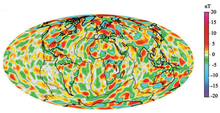
A model of short-wavelength features of Earth's magnetic field, attributed to lithospheric anomalies^[69]

Magnetometers observe minute deviations in the Earth's magnetic field caused past iron artifacts, kilns, some types of stone structures, and even ditches and middens in archaeological geophysics. Using magnetic instruments adapted from airborne magnetic anomaly detectors adult during Earth War 2 to detect submarines,^[70] the magnetic variations beyond the ocean floor have been mapped. Basalt — the iron-rich, volcanic rock making up the sea flooring^[71] — contains a strongly magnetic mineral (magnetite) and tin can locally distort compass readings. The baloney was recognized by Icelandic mariners as early as the late 18th century.^[72] More than important, because the presence of magnetite gives the basalt measurable magnetic properties, these magnetic variations have provided another means to study the deep ocean floor. When newly formed stone cools, such magnetic materials record the Earth's magnetic field.^[72]

Statistical models [edit]

Each measurement of the magnetic field is at a particular place and fourth dimension. If an authentic estimate of the field at some other place and time is needed, the measurements must be converted to a model and the model used to make predictions.

Spherical harmonics [edit]

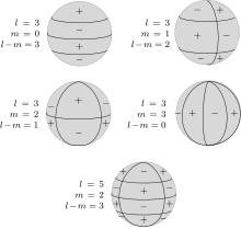
Schematic representation of spherical harmonics on a sphere and their nodal lines. $P ℓ m$ is equal to 0 forth $chiliad$ great circles passing through the poles, and along $ℓ- k$ circles of equal breadth. The role changes sign each ℓtime it crosses one of these lines.

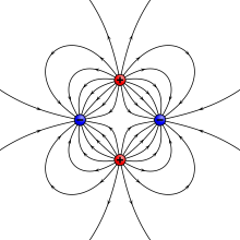
Instance of a quadrupole field. This can also be constructed past moving two dipoles together.

The about common mode of analyzing the global variations in the Earth's magnetic field is to fit the measurements to a set of spherical harmonics. This was starting time done by Carl Friedrich Gauss.^[73] Spherical harmonics are functions that oscillate over the surface of a sphere. They are the production of 2 functions, one that depends on latitude and one on longitude. The function of longitude is naught along zip or more than great circles passing through the North and South Poles; the number of such nodal lines is the accented value of the order $m$ . The office of latitude is zero along zero or more breadth circles; this plus the order is equal to the degree ℓ. Each harmonic is equivalent to a particular organization of magnetic charges at the center of the Earth. A monopole is an isolated magnetic charge, which has never been observed. A dipole is equivalent to ii opposing charges brought close together and a quadrupole to 2 dipoles brought together. A quadrupole field is shown in the lower figure on the right.^[12]

Spherical harmonics can represent any scalar field (function of position) that satisfies certain properties. A magnetic field is a vector field, only if it is expressed in Cartesian components $X, Y, Z$ , each component is the derivative of the aforementioned scalar role called the magnetic potential. Analyses of the Earth'southward magnetic field use a modified version of the usual spherical harmonics that differ by a multiplicative factor. A least-squares fit to the magnetic field measurements gives the World's field as the sum of spherical harmonics, each multiplied by the best-fitting Gauss coefficient $1000 m ℓ$ or $h chiliad ℓ$ .^[12]

The lowest-caste Gauss coefficient, $thousand 00$ , gives the contribution of an isolated magnetic charge, so it is zilch. The side by side iii coefficients – $g 10$ , $1000 ane 1$ , and $h ane ane$ – determine the direction and magnitude of the dipole contribution. The best fitting dipole is tilted at an bending of about ten° with respect to the rotational axis, every bit described before.^[12]

Radial dependence [edit]

Spherical harmonic analysis can be used to distinguish internal from external sources if measurements are available at more than one top (for example, ground observatories and satellites). In that example, each term with coefficient $1000 grand ℓ$ or $h grand ℓ$ can be split into two terms: ane that decreases with radius as $one/ r ℓ+1$ and one that increases with radius as $r ℓ$ . The increasing terms fit the external sources (currents in the ionosphere and magnetosphere). Still, averaged over a few years the external contributions average to zero.^[12]

The remaining terms predict that the potential of a dipole source ( $ℓ=1$ ) drops off equally $1/ r two$ . The magnetic field, being a derivative of the potential, drops off as $ane/ r 3$ . Quadrupole terms drib off equally $1/ r 4$ , and higher society terms drop off increasingly rapidly with the radius. The radius of the outer core is most half of the radius of the Earth. If the field at the core-mantle boundary is fit to spherical harmonics, the dipole office is smaller past a factor of about eight at the surface, the quadrupole part by a factor of 16, and so on. Thus, only the components with large wavelengths can be noticeable at the surface. From a variety of arguments, it is usually assumed that only terms upward to degree $14$ or less have their origin in the cadre. These have wavelengths of near 2,000 km (1,200 mi) or less. Smaller features are attributed to crustal anomalies.^[12]

Global models [edit]

The International Association of Geomagnetism and Aeronomy maintains a standard global field model called the International Geomagnetic Reference Field (IGRF). Information technology is updated every five years. The 11th-generation model, IGRF11, was developed using data from satellites (Ørsted, CHAMP and SAC-C) and a earth network of geomagnetic observatories.^[74] The spherical harmonic expansion was truncated at degree ten, with 120 coefficients, until 2000. Subsequent models are truncated at degree xiii (195 coefficients).^[75]

Another global field model, chosen the World Magnetic Model, is produced jointly by the United States National Centers for Environmental Information (formerly the National Geophysical Data Center) and the British Geological Survey. This model truncates at degree 12 (168 coefficients) with an judge spatial resolution of 3,000 kilometers. It is the model used by the The states Section of Defense, the Ministry building of Defence (Great britain), the U.s.a. Federal Aviation Administration (FAA), the North Atlantic Treaty Organization (NATO), and the International Hydrographic Arrangement as well as in many civilian navigation systems.^[76]

The in a higher place models simply have into account the "main field" at the core-mantle boundary. Although generally good enough for navigation, higher-accuracy apply cases require smaller-scale magnetic anomalies and other variations to be considered. Some examples are (see geomag.the states ref for more than):^[77]

The "comprehensive modeling" (CM) appproach past the Goddard Space Flight Heart (NASA and GSFC) and the Danish Space Research Institute. CM attempts to reconcile information with greatly varying temporal and spatial resolution from ground and satellite sources. The latest version as of 2022 is CM5 of 2016. Information technology provides separate components for principal field plus lithosphere (crustal), M2 tidal, and principal/induced magnetosphere/ionosphere variations.^[78]
The Us National Centers for Environmental Information developed the Enhanced Magnetic Model (EMM), which extends to degree and lodge 790 and resolves magnetic anomalies downwardly to a wavelength of 56 kilometers. It was compiled from satellite, marine, aeromagnetic and ground magnetic surveys. As of 2018^[update], the latest version, EMM2017, includes data from The European Space Agency's Swarm satellite mission.^[79]

For historical information virtually the main field, the IGRF may be used back to year 1900.^[75] A specialized GUFM1 model estimates dorsum to year 1590 using ship's logs.^[80] Paleomagnetic research has produced models dating dorsum to 10,000 BCE.^[81]

Biomagnetism [edit]

Animals, including birds and turtles, can observe the Earth'south magnetic field, and use the field to navigate during migration.^[82] Some researchers have found that cows and wild deer tend to align their bodies north–southward while relaxing, but not when the animals are under high-voltage power lines, suggesting that magnetism is responsible.^[83] ^[84] Other researchers reported in 2011 that they could not replicate those findings using different Google Earth images.^[85]

Very weak electromagnetic fields disrupt the magnetic compass used by European robins and other songbirds, which use the World's magnetic field to navigate. Neither power lines nor cellphone signals are to blame for the electromagnetic field consequence on the birds;^[86] instead, the culprits have frequencies between 2 kHz and 5 MHz. These include AM radio signals and ordinary electronic equipment that might exist found in businesses or private homes.^[87]

See as well [edit]

Geomagnetic jerk
Geomagnetic latitude
Magnetic field of Mars
Magnetotellurics
Operation Argus

References [edit]

^ ^a ^b Glatzmaier, Gary A.; Roberts, Paul H. (1995). "A three-dimensional self-consistent figurer simulation of a geomagnetic field reversal". Nature. 377 (6546): 203–209. Bibcode:1995Natur.377..203G. doi:10.1038/377203a0. S2CID 4265765.
^ Glatzmaier, Gary. "The Geodynamo". University of California Santa Cruz. Retrieved 20 October 2013.
^ Finlay, C. C.; Maus, Southward.; Beggan, C. D.; Bondar, T. Northward.; Chambodut, A.; Chernova, T. A.; Chulliat, A.; Golovkov, Five. P.; Hamilton, B.; Hamoudi, M.; Holme, R.; Hulot, Chiliad.; Kuang, W.; Langlais, B.; Lesur, V.; Lowes, F. J.; Lühr, H.; Macmillan, S.; Mandea, Thousand.; McLean, Southward.; Manoj, C.; Menvielle, K.; Michaelis, I.; Olsen, N.; Rauberg, J.; Rother, K.; Sabaka, T. J.; Tangborn, A.; Tøffner-Clausen, L.; Thébault, Eastward.; Thomson, A. W. P.; Wardinski, I.; Wei, Z.; Zvereva, T. I. (December 2010). "International Geomagnetic Reference Field: the eleventh generation". Geophysical Journal International. 183 (3): 1216–1230. Bibcode:2010GeoJI.183.1216F. doi:10.1111/j.1365-246X.2010.04804.x.
^ Shlermeler, Quirin (iii March 2005). "Solar current of air hammers the ozone layer". News@nature. doi:10.1038/news050228-12.
^ "Solar wind ripping chunks off Mars". Cosmos Online. 25 Nov 2008. Archived from the original on 4 March 2016. Retrieved 21 Oct 2013.
^ Luhmann, Johnson & Zhang 1992 harvnb error: no target: CITEREFLuhmannJohnsonZhang1992 (help)
^ Structure of the World Archived 2013-03-15 at the Wayback Machine. Scign.jpl.nasa.gov. Retrieved on 2012-01-27.
^ ^a ^b ^c ^d McElhinny, Michael W.; McFadden, Phillip 50. (2000). Paleomagnetism: Continents and Oceans. Bookish Press. ISBN978-0-12-483355-5.
^ Opdyke, Neil D.; Channell, James E. T. (1996). Magnetic Stratigraphy. Academic Press. ISBN978-0-12-527470-8.
^ Mussett, Alan Eastward.; Khan, Thou. Aftab (2000). Looking into the Earth: An introduction to Geological Geophysics. Cambridge University Press. ISBN978-0-521-78085-8.
^ Temple, Robert (2006). The Genius of China. Andre Deutsch. ISBN978-0-671-62028-8.
^ ^a ^b ^c ^d ^eastward ^f ^g ^h ⁱ ^j Merrill, McElhinny & McFadden 1996, Chapter ii
^ ^a ^b "Geomagnetism Frequently Asked Questions". National Geophysical Data Middle. Retrieved 21 October 2013.
^ Palm, Eric (2011). "Tesla". National Loftier Magnetic Field Laboratory. Archived from the original on 21 March 2013. Retrieved xx October 2013.
^ ^a ^b Chulliat, A.; Macmillan, South.; Alken, P.; Beggan, C.; Nair, Thou.; Hamilton, B.; Forest, A.; Ridley, V.; Maus, S.; Thomson, A. (2015). The United states of america/UK World Magnetic Model for 2015-2020 (PDF) (Report). National Geophysical Data Heart. Retrieved 21 February 2016.
^ "Ancient lava reveals secrets of Earth's magnetic field cycle". Cosmos Magazine. 2021-08-31. Retrieved 2021-09-03 .
^ Casselman, Anne (28 February 2008). "The Earth Has More Than One North Pole". Scientific American . Retrieved 21 May 2013.
^ Serway, Raymond A.; Chris Vuille (2006). Essentials of higher physics. U.s.: Cengage Learning. p. 493. ISBN978-0-495-10619-vii.
^ Emiliani, Cesare (1992). Planet Earth: Cosmology, Geology, and the Development of Life and Environment. Great britain: Cambridge University Press. p. 228. ISBN978-0-521-40949-0.
^ Manners, Joy (2000). Static Fields and Potentials. USA: CRC Press. p. 148. ISBN978-0-7503-0718-5.
^ Nave, Carl R. (2010). "Bar Magnet". Hyperphysics. Dept. of Physics and Astronomy, Georgia State Univ. Retrieved 2011-04-10 .
^ Campbell, Wallace A. (1996). ""Magnetic" pole locations on global charts are incorrect". Eos, Transactions American Geophysical Union. 77 (36): 345. Bibcode:1996EOSTr..77..345C. doi:10.1029/96EO00237. S2CID 128421452.
^ "The Magnetic North Pole". Woods Hole Oceanographic Establishment. Archived from the original on 19 August 2013. Retrieved 21 October 2013.
^ ^a ^b ^c Phillips, Tony (29 Dec 2003). "Globe's Inconstant Magnetic Field". Science@Nasa . Retrieved 27 December 2009.
^ ^a ^b ^c ^d ^e Merrill 2010, pages 126–141
^ ^a ^b ^c Parks, George K. (1991). Physics of space plasmas: an introduction. Redwood City, Calif.: Addison-Wesley. ISBN978-0201508215.
^ Darrouzet, Fabien; De Keyser, Johan; Escoubet, C. Philippe (ten September 2013). "Cluster shows plasmasphere interacting with Van Allen belts" (Press release). European Space Agency. Retrieved 22 October 2013.
^ "Shields Upward! A breeze of interstellar helium atoms is bravado through the solar system". Science@NASA. 27 September 2004. Retrieved 23 October 2013.
^ Odenwald, Sten (2010). "The great solar superstorm of 1859". Applied science Through Fourth dimension. 70. Archived from the original on 12 October 2009. Retrieved 24 October 2013.
^ "The K-index". Space Weather condition Prediction Center. Archived from the original on 22 October 2013. Retrieved 20 October 2013.
^ Steigerwald, Bill (xvi Dec 2008). "Lord's day Often "Tears Out A Wall" In Earth's Solar Storm Shield". THEMIS: Understanding space weather. NASA. Retrieved 20 Baronial 2011.
^ Jackson, Andrew; Jonkers, Fine art R. T.; Walker, Matthew R. (2000). "4 centuries of Geomagnetic Secular Variation from Historical Records". Philosophical Transactions of the Purple Club A. 358 (1768): 957–990. Bibcode:2000RSPTA.358..957J. CiteSeerX10.1.ane.560.5046. doi:ten.1098/rsta.2000.0569. JSTOR 2666741. S2CID 40510741.
^ ^a ^b "Secular variation". Geomagnetism. Canadian Geological Survey. 2011. Archived from the original on 25 July 2008. Retrieved 18 July 2011.
^ Constable, Catherine (2007). "Dipole Moment Variation". In Gubbins, David; Herrero-Bervera, Emilio (eds.). Encyclopedia of Geomagnetism and Paleomagnetism. Springer-Verlag. pp. 159–161. doi:10.1007/978-1-4020-4423-6_67. ISBN978-one-4020-3992-8.
^ Dumberry, Mathieu; Finlay, Christopher C. (2007). "Eastward and westward drift of the Earth's magnetic field for the last three millennia" (PDF). Earth and Planetary Scientific discipline Letters. 254 (one–two): 146–157. Bibcode:2007E&PSL.254..146D. doi:10.1016/j.epsl.2006.11.026. Archived from the original (PDF) on 2013-10-23. Retrieved 2013-x-22 .
^ Tauxe 1998, Chapter 1
^ "Simulations show magnetic field can change 10 times faster than previously idea". phys.org . Retrieved xvi August 2020.
^ Davies, Christopher J.; Constable, Catherine G. (6 July 2020). "Rapid geomagnetic changes inferred from Earth observations and numerical simulations". Nature Communications. 11 (i): 3371. Bibcode:2020NatCo..eleven.3371D. doi:10.1038/s41467-020-16888-0. ISSN 2041-1723. PMC7338531. PMID 32632222.
^ Coe, R. Due south.; Prévot, Thousand.; Camps, P. (xx April 1995). "New evidence for extraordinarily rapid alter of the geomagnetic field during a reversal". Nature. 374 (6524): 687–692. Bibcode:1995Natur.374..687C. doi:10.1038/374687a0. S2CID 4247637. (also bachelor online at es.ucsc.edu)
^ Coe, R. Southward.; Jarboe, N. A.; Le Goff, M.; Petersen, N. (15 August 2014). "Demise of the rapid-field-change hypothesis at Steens Mountain: The crucial function of continuous thermal demagnetization". Earth and Planetary Science Letters. 400: 302–312. Bibcode:2014E&PSL.400..302C. doi:10.1016/j.epsl.2014.05.036.
^ Vacquier, Victor (1972). Geomagnetism in marine geology (2d ed.). Amsterdam: Elsevier Scientific discipline. p. 38. ISBN9780080870427.
^ Merrill, McElhinny & McFadden 1996, Chapter v
^ Merrill, McElhinny & McFadden 1996, pp. 148–155
^ Nowaczyk, North. R.; Arz, H. Due west.; Frank, U.; Kind, J.; Plessen, B. (16 October 2012). "Ice Age Polarity Reversal Was Global Consequence: Extremely Brief Reversal of Geomagnetic Field, Climate Variability, and Super Volcano". Earth and Planetary Science Messages. 351: 54. Bibcode:2012E&PSL.351...54N. doi:10.1016/j.epsl.2012.06.050. Retrieved 21 March 2013.
^ McElhinney, T. N. Due west.; Senanayake, W. E. (1980). "Paleomagnetic Bear witness for the Existence of the Geomagnetic Field iii.5 Ga Ago". Periodical of Geophysical Research. 85 (B7): 3523. Bibcode:1980JGR....85.3523M. doi:ten.1029/JB085iB07p03523.
^ Usui, Yoichi; Tarduno, John A.; Watkeys, Michael; Hofmann, Axel; Cottrell, Rory D. (2009). "Evidence for a 3.45-billion-twelvemonth-old magnetic remanence: Hints of an ancient geodynamo from conglomerates of South Africa". Geochemistry, Geophysics, Geosystems. 10 (nine): northward/a. Bibcode:2009GGG....1009Z07U. doi:x.1029/2009GC002496.
^ Tarduno, J. A.; Cottrell, R. D.; Watkeys, M. K.; Hofmann, A.; Doubrovine, P. 5.; Mamajek, E. E.; Liu, D.; Sibeck, D. M.; Neukirch, L. P.; Usui, Y. (four March 2010). "Geodynamo, Solar Air current, and Magnetopause 3.4 to 3.45 Billion Years Agone". Scientific discipline. 327 (5970): 1238–1240. Bibcode:2010Sci...327.1238T. doi:10.1126/science.1183445. PMID 20203044. S2CID 23162882.
^ Lovett, Richard A. (December 24, 2009). "Northward Magnetic Pole Moving Due to Cadre Flux".
^ Witze, Alexandra (9 January 2019). "Earth's magnetic field is interim up and geologists don't know why". Nature. 565 (7738): 143–144. Bibcode:2019Natur.565..143W. doi:10.1038/d41586-019-00007-1. PMID 30626958.
^ "How does the Earth'southward core generate a magnetic field?". USGS FAQs. The states Geological Survey. Archived from the original on 18 January 2015. Retrieved 21 October 2013.
^ ^a ^b Weiss, Nigel (2002). "Dynamos in planets, stars and galaxies". Astronomy and Geophysics. 43 (3): 3.09–3.fifteen. Bibcode:2002A&G....43c...9W. doi:10.1046/j.1468-4004.2002.43309.x.
^ Jordan, T. H. (1979). "Structural Geology of the Earth's Interior". Proceedings of the National Academy of Sciences. 76 (9): 4192–4200. Bibcode:1979PNAS...76.4192J. doi:x.1073/pnas.76.9.4192. PMC411539. PMID 16592703.
^ European Synchrotron Radiation Facility (25 Apr 2013). "Earth'due south Middle Is 1,000 Degrees Hotter Than Previously Thought, Synchrotron 10-Ray Experiment Shows". ScienceDaily . Retrieved 21 Oct 2013.
^ ^a ^b Buffett, B. A. (2000). "Earth's Core and the Geodynamo". Science. 288 (5473): 2007–2012. Bibcode:2000Sci...288.2007B. doi:x.1126/science.288.5473.2007. PMID 10856207.
^ Feynman, Richard P. (2010). The Feynman lectures on physics (New millennium ed.). New York: BasicBooks. pp. 13–3, 15–14, 17–2. ISBN9780465024940.
^ ^a ^b ^c ^d ^e Merrill, McElhinny & McFadden 1996, Chapter 8
^ Merrill, McElhinny & McFadden 1996, Chapter ten
^ Merrill, McElhinny & McFadden 1996, Chapter 11
^
Buffett, Bruce A. (2010). "Tidal dissipation and the strength of the Globe's internal magnetic field". Nature. 468 (7326): 952–954. Bibcode:2010Natur.468..952B. doi:10.1038/nature09643. PMID 21164483. S2CID 4431270.
- "Commencement Measurement Of Magnetic Field Within Earth'due south Core". Science 20. December 17, 2010.
^ ^a ^b Kono, Masaru; Roberts, Paul H. (2002). "Recent geodynamo simulations and observations of the geomagnetic field". Reviews of Geophysics. 40 (iv): 1–53. Bibcode:2002RvGeo..40.1013K. doi:10.1029/2000RG000102. S2CID 29432436.
^ Kageyama, Akira; Sato, Tetsuya; the Complexity Simulation Group (1 January 1995). "Computer simulation of a magnetohydrodynamic dynamo. Ii". Physics of Plasmas. 2 (5): 1421–1431. Bibcode:1995PhPl....two.1421K. doi:x.1063/1.871485.
^ Glatzmaier, Gary A.; Roberts, Paul H. (1995). "A three-dimensional convective dynamo solution with rotating and finitely conducting inner core and mantle". Physics of the Globe and Planetary Interiors. 91 (1–3): 63–75. Bibcode:1995PEPI...91...63G. doi:10.1016/0031-9201(95)03049-3.
^ ^a ^b ^c "Bounding main Tides and Magnetic Fields". NASA. Scientific Visualization Studio. 2016-12-30. This article incorporates text from this source, which is in the public domain.
^ Irrgang, Christopher; Saynisch, January; Thomas, Maik (2019). "Estimating global sea heat content from tidal magnetic satellite observations". Scientific Reports. 9 (one): 7893. Bibcode:2019NatSR...nine.7893I. doi:x.1038/s41598-019-44397-viii. PMC6536534. PMID 31133648.
^ Stepišnik, Janez (2006). "Spectroscopy: NMR downwards to Globe". Nature. 439 (7078): 799–801. Bibcode:2006Natur.439..799S. doi:10.1038/439799a. PMID 16482144.
^ Gauss, C.F (1832). "The Intensity of the Earth's Magnetic Strength Reduced to Accented Measurement" (PDF) . Retrieved 2009-x-21 .
^ Courtillot, Vincent; Le Mouel, Jean Louis (1988). "Time Variations of the Globe's Magnetic Field: From Daily to Secular". Almanac Review of Earth and Planetary Sciences. 1988 (16): 435. Bibcode:1988AREPS..xvi..389C. doi:ten.1146/annurev.ea.sixteen.050188.002133.
^ Hulot, G.; Eymin, C.; Langlais, B.; Mandea, M.; Olsen, N. (April 2002). "Small-scale-scale construction of the geodynamo inferred from Oersted and Magsat satellite data". Nature. 416 (6881): 620–623. Bibcode:2002Natur.416..620H. doi:10.1038/416620a. PMID 11948347. S2CID 4426588.
^ Frey, Herbert. "Satellite Magnetic Models". Comprehensive Modeling of the Geomagnetic Field. NASA. Retrieved 13 Oct 2011.
^ William F. Hanna (1987). Geologic Applications of Modern Aeromagnetic Surveys (PDF). USGS. p. 66. Retrieved three May 2017.
^ G. D. Nicholls (1965). "Basalts from the Deep Body of water Flooring" (PDF). Mineralogical Magazine. 34 (268): 373–388. Bibcode:1965MinM...34..373N. doi:10.1180/minmag.1965.034.268.32. Archived from the original (PDF) on xvi July 2017. Retrieved 3 May 2017.
^ ^a ^b Jacqueline Westward. Kious; Robert I. Tilling (1996). This Dynamic Globe: The Story of Plate Tectonics. USGS. p. 17. ISBN978-0160482205 . Retrieved iii May 2017.
^ Campbell 2003, p. 1.
^ Finlay, CC; Maus, S; Beggan, CD; Hamoudi, M.; Lowes, FJ; Olsen, N; Thébault, E. (2010). "Evaluation of candidate geomagnetic field models for IGRF-11" (PDF). Earth, Planets and Space. 62 (ten): 787–804. Bibcode:2010EP&Southward...62..787F. doi:x.5047/eps.2010.11.005. S2CID 530534.
^ ^a ^b "The International Geomagnetic Reference Field: A "Health" Alarm". National Geophysical Data Eye. January 2010. Retrieved 13 October 2011.
^ "The World Magnetic Model". National Geophysical Information Center. Retrieved 14 October 2011.
^ "Geomagnetic and Electric Field Models". geomag.us.
^ "Model data". ccmc.gsfc.nasa.gov.
^ "The Enhanced Magnetic Model". United States National Centers for Environmental Information. Retrieved 29 June 2018.
^ Jackson, Andrew; Jonkers, Art R. T.; Walker, Matthew R. (15 March 2000). "Four centuries of geomagnetic secular variation from historical records". Philosophical Transactions of the Majestic Order of London. Serial A: Mathematical, Physical and Engineering Sciences. 358 (1768): 957–990. Bibcode:2000RSPTA.358..957J. doi:10.1098/rsta.2000.0569. S2CID 40510741.
^ "The GEOMAGIA database". geomagia.gfz-potsdam.de.
^ Deutschlander, K.; Phillips, J.; Borland, S. (1999). "The case for light-dependent magnetic orientation in animals". Journal of Experimental Biological science. 202 (8): 891–908. doi:ten.1242/jeb.202.viii.891. PMID 10085262.
^ Burda, H.; Begall, S.; Cerveny, J.; Neef, J.; Nemec, P. (2009). "Extremely depression-frequency electromagnetic fields disrupt magnetic alignment of ruminants". Proceedings of the National Academy of Sciences. 106 (14): 5708–xiii. Bibcode:2009PNAS..106.5708B. doi:10.1073/pnas.0811194106. PMC2667019. PMID 19299504.
^ "Biological science: Electric cows". Nature. 458 (7237): 389. 2009. Bibcode:2009Natur.458Q.389.. doi:ten.1038/458389a.
^ Hert, J; Jelinek, 50; Pekarek, L; Pavlicek, A (2011). "No alignment of cattle along geomagnetic field lines institute". Journal of Comparative Physiology. 197 (6): 677–682. arXiv:1101.5263. doi:10.1007/s00359-011-0628-seven. PMID 21318402. S2CID 15520857. [i]
^ Engels, Svenja; Schneider, Nils-Lasse; Lefeldt, Nele; Hein, Christine Maira; Zapka, Manuela; Michalik, Andreas; Elbers, Dana; Kittel, Achim; Hore, P. J. (2014-05-15). "Anthropogenic electromagnetic noise disrupts magnetic compass orientation in a migratory bird". Nature. 509 (7500): 353–356. Bibcode:2014Natur.509..353E. doi:10.1038/nature13290. ISSN 0028-0836. PMID 24805233. S2CID 4458056.
^ Hsu, Jeremy (9 May 2014). "Electromagnetic Interference Disrupts Bird Navigation, Hints at Quantum Action". IEEE Spectrum . Retrieved 31 May 2015.

External links [edit]

Geomagnetism & Paleomagnetism background material Archived 2013-03-03 at the Wayback Machine. American Geophysical Matrimony Geomagnetism and Paleomagnetism Department.
National Geomagnetism Plan. United States Geological Survey, March 8, 2011.
BGS Geomagnetism. Data on monitoring and modeling the geomagnetic field. British Geological Survey, August 2005.
William J. Broad, Volition Compasses Indicate South?. The New York Times, July xiii, 2004.
John Roach, Why Does Earth's Magnetic Field Flip?. National Geographic, September 27, 2004.
Magnetic Tempest. PBS NOVA, 2003. (ed. about pole reversals)
When North Goes South. Projects in Scientific Computing, 1996.
The Bully Magnet, the Earth, History of the discovery of Earth's magnetic field by David P. Stern.
Exploration of the Earth'south Magnetosphere Archived 2013-02-14 at the Wayback Machine, Educational web site past David P. Stern and Mauricio Peredo
International Geomagnetic Reference Field 2011
Global evolution/anomaly of the Earth's magnetic field Archived 2016-06-24 at the Wayback Machine Sweeps are in 10° steps at 10 years intervals. Based on information from: The Found of Geophysics, ETH Zurich Archived 2007-ten-31 at the Wayback Machine
Patterns in Globe'south magnetic field that evolve on the order of one,000 years Archived 2018-07-xx at the Wayback Automobile. July xix, 2017
Chree, Charles (1911). "Magnetism, Terrestrial". In Chisholm, Hugh (ed.). Encyclopædia Britannica. Vol. 17 (11th ed.). Cambridge University Press. pp. 353–385. (with dozens of tables and several diagrams)